did you MNIST me?
March 05, 2026
Yep. I’m back. And blogging again. It’s been a while. I forgot how to write introductions, so let’s just get started with the fun stuff.
You might be wondering what on earth I did to my GAN to get it to produce something like that. Let me explain: When stable diffusion first came out, I thought it was pretty sick. It’s hard to wrap your head around what kind of math is behind that stuff. I wanted to find out for myself, and the best way to learn about something is to build it. It wasn’t until I started looking into this that I learned that there was a long history of trial and error in image generation. Here’s some things I did to explore further.
training a CNN classifier
What is a CNN? From my understanding, it’s a specialized type of neural network that’s good at processing grid-like data (like images!). It does so using convolutions.
huh
Convolution is a mathematical operation that applies a kernel over an input. Think of it like moving a smaller grid over a bigger grid, multiplying the numbers in the grid that overlap. You can change the small grid to extract certain things from the bigger grid. For example, if the bigger grid is an image, you can extract features like edges, lines, and more.
what I did
- I designed the forward pass through the CNN as such:
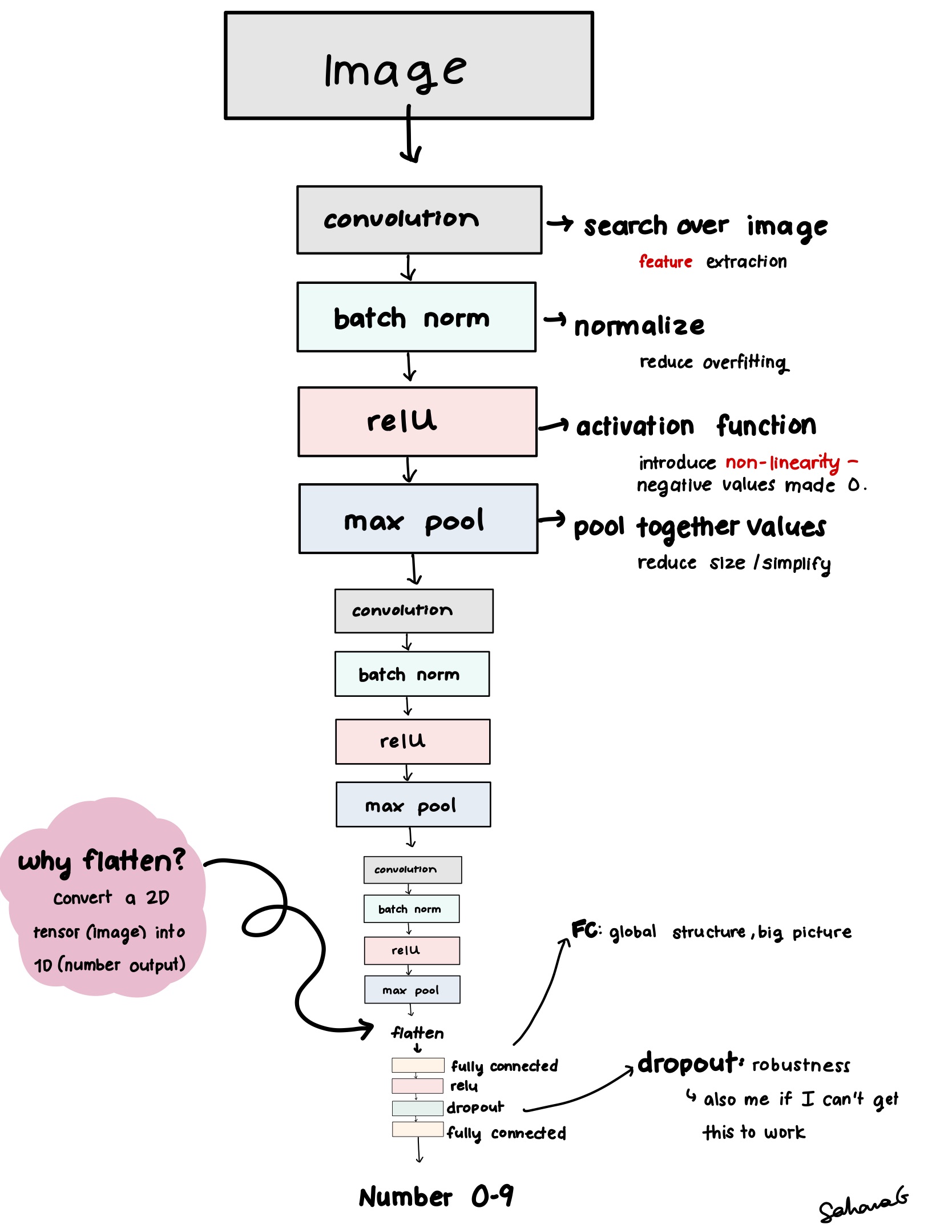 Results:
Overall Accuracy: 98.69%
Accuracy of digit 0: 99.39%
Accuracy of digit 1: 99.56%
Accuracy of digit 2: 97.77%
Accuracy of digit 3: 99.11%
Accuracy of digit 4: 99.69%
Accuracy of digit 5: 97.42%
Accuracy of digit 6: 98.12%
Accuracy of digit 7: 99.03%
Accuracy of digit 8: 99.49%
Accuracy of digit 9: 97.13%
Thoughts: It performed very well. This is most likely because of what I explained earlier: Convolution is great for handling grid like data with patterns like images of digits. More complicated images might give this neural net some problems.
training a GAN to generate handwritten letters and numbers
(and why people don’t use GANs anymore)
How does a GAN work? A GAN stands for generative adversarial network made of two components, and it functions like your typical divorced household. You are a child in a broken home, and two parents are constantly trying to one-up each other to win your love.
- The Generator takes in noise, outputs a sample.
- The Discriminator (I did not come up with this name.) takes in both real images and generated ones and outputs a binary “real” or “fake” score.
- The generator gets upset and says the discriminator doesn’t know what they’re talking about anyway since they missed your ballet recital last week.
- Just kidding. The generator updates its weights. So does the discriminator! They get better at attacking each other.
- unstable as hell (wonder why.)
The Original GAN paper explains the theory behind why eventually, the generator will begin to make samples that are pretty much indistinguishable from real data, so the discriminator accuracy hits 50% (where it is basically just guessing randomly. Can relate.)
what I did:
Discriminator architecture
The discriminator can be simplified into a binary classifier, so it would be similar to the CNN classifier I made earlier.
- Instead of outputting a probability score between 0 and 1 for each number, it would output a single probability between 0 and 1: The probability that this image is real.
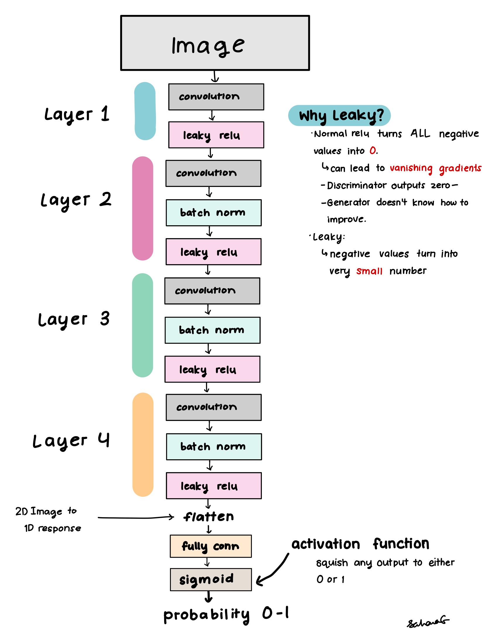
The forward pass for the discriminator is like so:
Generator architecture
The generator is basically an inverse classifier.
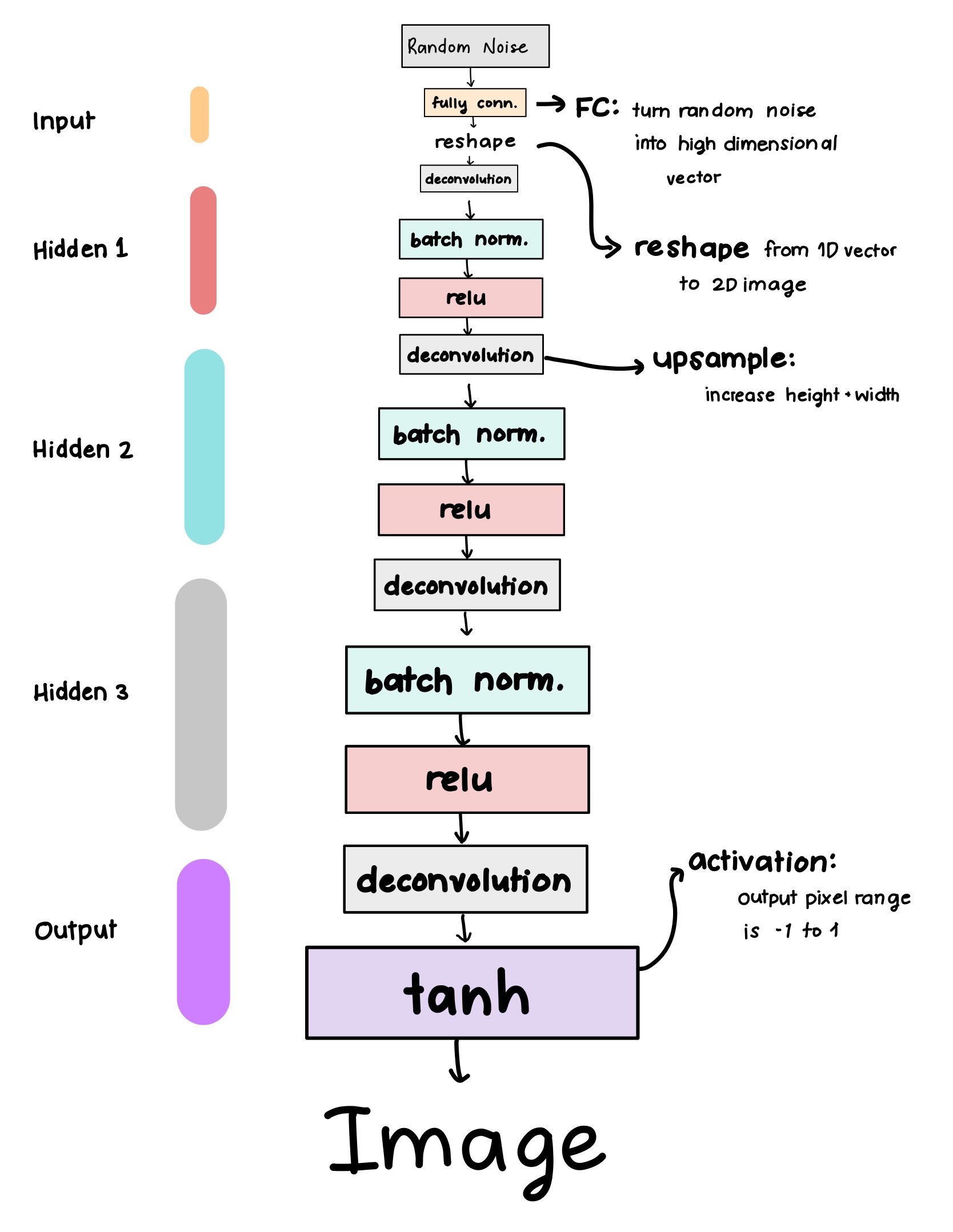
- We use one linear layer to upsample to reasonable shape of a small image
- Then reshape to an actual image tensor
Instead of taking in an image, we take in a random vector from a latent space representing the dataset (normal or uniform distribution). Basically just random noise with compressed pieces of edges and lines you might see in MNIST.
I made the forward pass through the generator like so:
One thing that was tricky was weight initialization, since GANs are sensitive to that. Weight initialization is very important for stable training. If we do this wrong, the GAN will throw a fit (mode collapse, exploding gradients, or just not learning anything. Kids these days).
- I used a normal distribution initialization for convolution, batchnorm, and linear layers
Existing Literature recommends pulling from a normal distribution between 0 and 0.2 for convolutional layers, while pulling from 1 and 0.2 for batch norm layers.
training loop
I started by training the discriminator on real data (real_images)
real_predictions = discriminator(real_images).view(-1)
d_loss_real = criterion(real_predictions, real_labels)
Then we get the loss on fake images generated by the generator (fake_img)
- We combine the loss on real and fake images to train the discriminator.
fake_predictions = discriminator(fake_img.detach()).view(-1)
d_loss_fake = criterion(fake_predictions, fake_labels)
The generator loss is based on its ability to fool the discriminator:
g_loss = criterion(fake_predictions, real_labels)
results
Good grief those loss curves are a BLOODBATH.
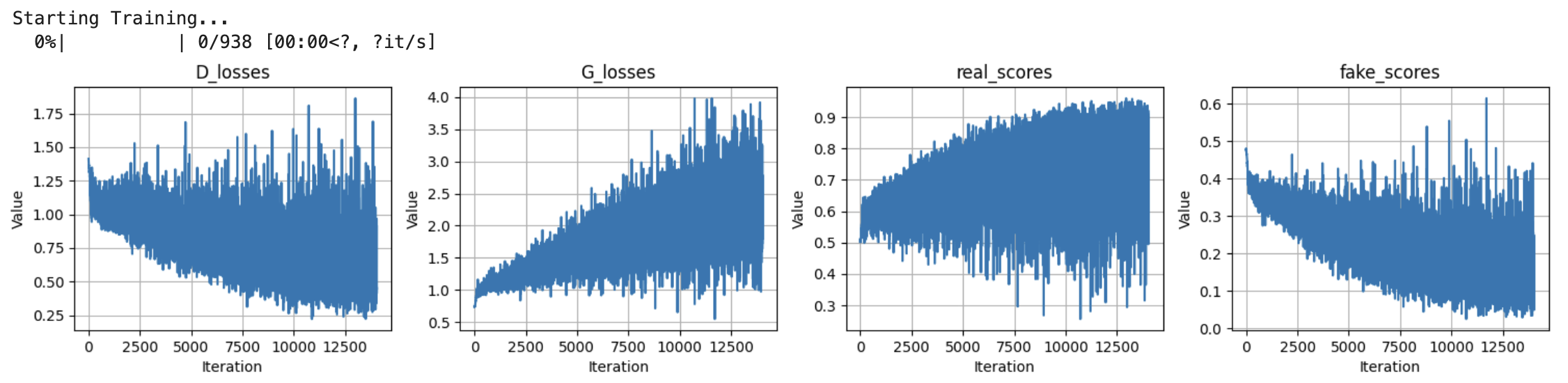
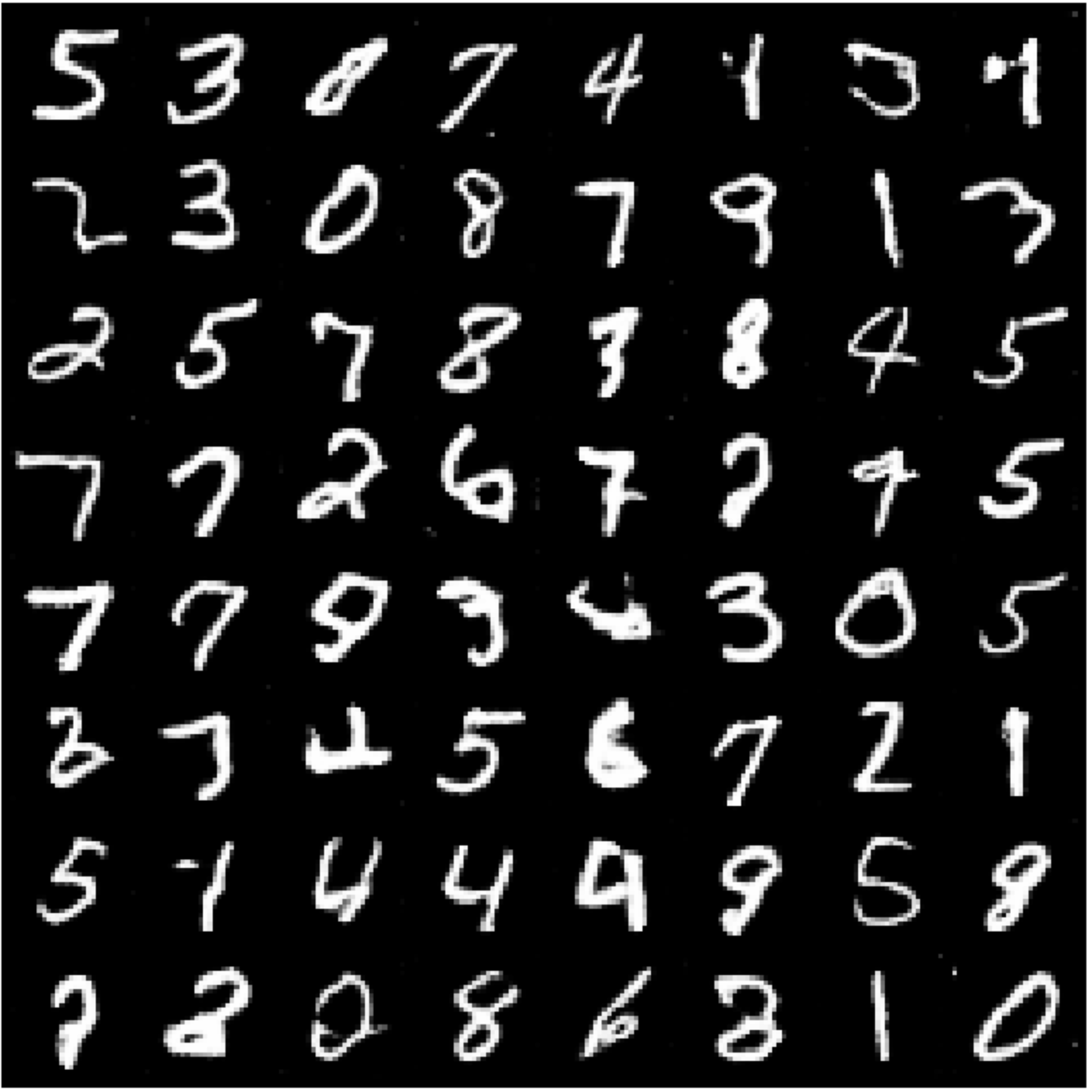
As you can see, those losses go crazy as the G and D duke it out, but the numbers don’t come out too bad.
- Took 8 hours to train just to look like someone with two left feet for hands wrote them. But oh well, such is life
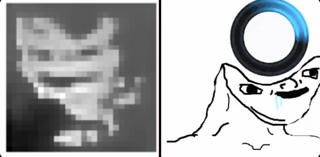
Notes: training takes forever, and extra work is done figuring out how to initialize the weights so that it doesn’t flip out on me. While I was having trouble with weights initialization, I got these images:
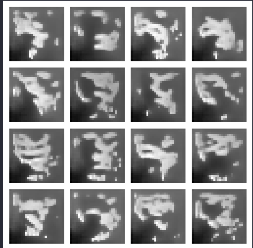
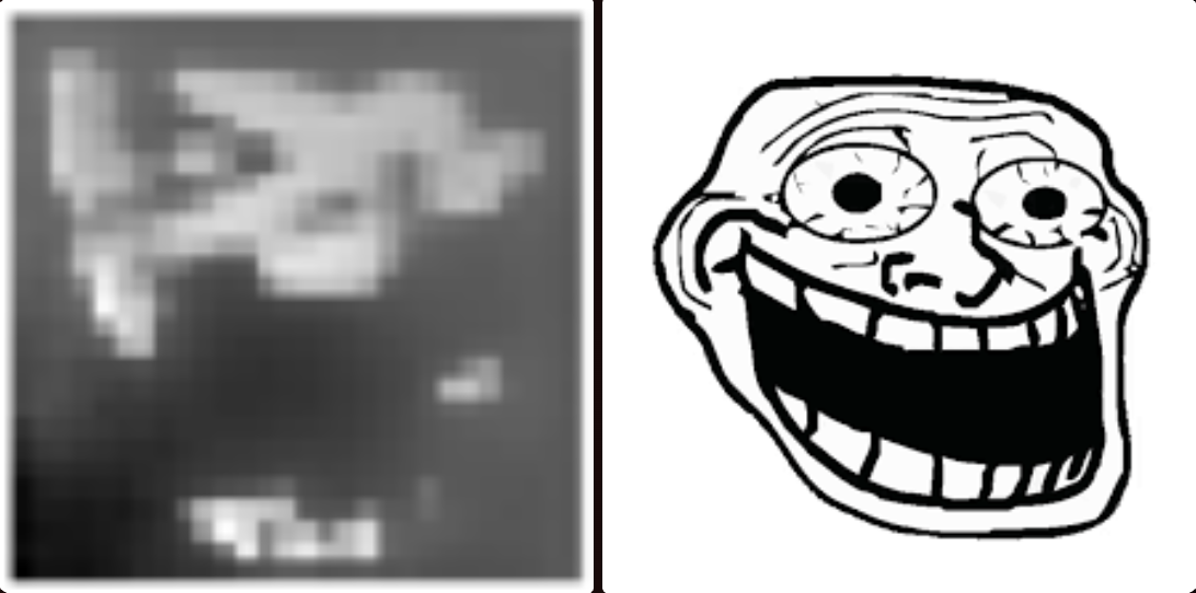
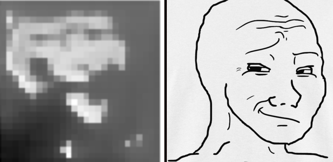
- This thing has the humor of a gen alpha iPad kid. What have I created
training a Diffusion model to do the same thing
and why people love diffusion models
How does diffusion work? First, we take a clean image.
- The forward process gradually adds noise over time to the image
- Eventually the image just becomes pure noise.
- A neural net is trained to predict noise added at each timestep in the forward process
- Then, the reverse process (generation) starts from noise and gradually removes it.
- Since we learned to predict what noise was added, we know how to denoise it.
Here’s the original paper. for DDPM (Denoising Diffusion Probabilistic Models).
U-Net architecture
The U-Net is the combination of this forward and reverse process, named for looking like a “U” shape. Here’s a diagram showing this:
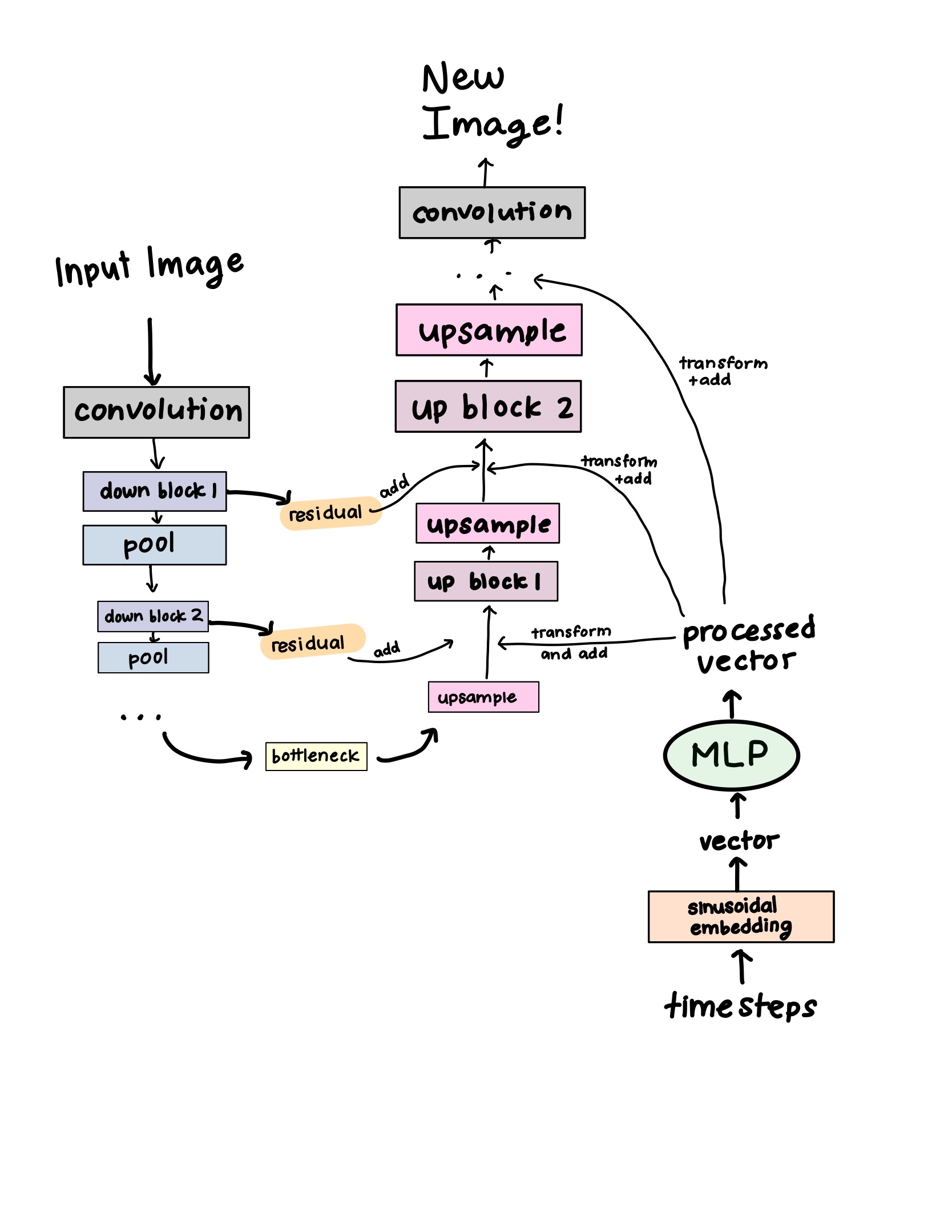
forward “down” pass
- The initial convolution projects the input image into a feature space
- Run it through downblocks, where each one
- applies a convolution layer, saves the output as a residual (skip connection)
- downsamples with pooling
Why? This is so that we can extract high level, coarse grained features from the image. The bottleneck at the very end is how the model learns the global structure; the most compressed representation of the image.
time embedding
This is meant to tell the network where in the diffusion process it’s at. This is so that the model can tell if it’s early or late in the denoising process
- Convert the timestep t into a vector via sinusoidal embedding
- This embedding type is especially useful for encoding time/where in the process a step is. It’s also used in NLP
- Transform that vector with an MLP
- No, not My Little Pony. As much as I would like to ask Twilight Sparkle to fix my code, I go to UT Austin, not Equestria High. 😔
- Multi-Layer Perceptron: A tiny fully connected neural network that is just linear layers and SiLU.
- The point of it is to transform the embedding vector’s size (see the up pass for more details)
reverse “up” pass
- Upsample (gradually restore the resolution to the input image’s original size)
- Transform the time embedding vector to match the size of the upsampled
- We do this using the MLP I mentioned earlier!
- Now that the sizes match, we can concatenate the time embedding vector to that output
- Concatenate the residual from the matching downblock to the combined time embedding vector and upsampled output
- Well, now what are these for??
- As we downsample to learn global features, we lose fine-grained features. But what if we want to keep those?
- The down blocks save these features, so we can just concatenate them back in when upsampling. This preserves the fine detail (edges, textures) that might have been lost during the forward pass.
- Run it through an upblock
- What do these do? Well… we DID just haphazardly throw a bunch of information into a bowl like a low quality salad. It’s messy and unreadable, and our model is a bit of a picky eater.
- In the up block, convolution, normalization, and activation layers help to clean this up and fuse the features together.
- Repeat steps 2-4 for each upblock
- Final convolution: map the features back to the image space
objective
Via all of this, the network gradually learns to predict noise added given a noisy image and a timestep, and therefore how to remove the noise step-by-step.
training
First, I define a noise schedule, which helps determine how much noise is added at each step of the diffusion process. This is very important for training.
- The
betascontrol the amount of noise added at each step, while thealphacontrols how much of the previous step we want to preserve. - We take the cumulative product of all the alphas to see how much of the original image manages to make it to the end.
- Just like squid game
self.betas = torch.linspace(beta_start, beta_end, noise_steps).to(device)
self.alphas = 1. - self.betas
self.alpha_cumprod = torch.cumprod(self.alphas, dim=0)
During training, we do the forward process by adding noise to the real images.
tsac = self.sqrt_alpha_cumprod[t].view(-1, 1, 1, 1)
toms = self.one_min_sqrt[t].view(-1, 1, 1, 1)
noise = torch.rand_like(x)
noisy_images = tsac * x + toms * noise
The model takes in the noisy image and the timestep and tries to predict the noise that was added.
pred_noise = self.model(noisy_images, t)
loss = F.mse_loss(pred_noise, noise)
reverse process
We create random noise. Then, we get the model to predict what noise was added, and subtract that estimate. Repeat this enough, and we should hopefully get a clean image!
x = torch.randn(num_samples, self.model.channels, self.model.image_size, self.model.image_size)
# go thru timesteps in reverse
for i in reversed(range(self.noise_steps)):
	pred_noise = self.model(x, t)
	x = 1 / torch.sqrt(alpha) * (x - (beta / torch.sqrt(1 - alpha_cumprod)) * pred_noise) + torch.sqrt(beta) * noise
and now, what you were waiting for. The results!
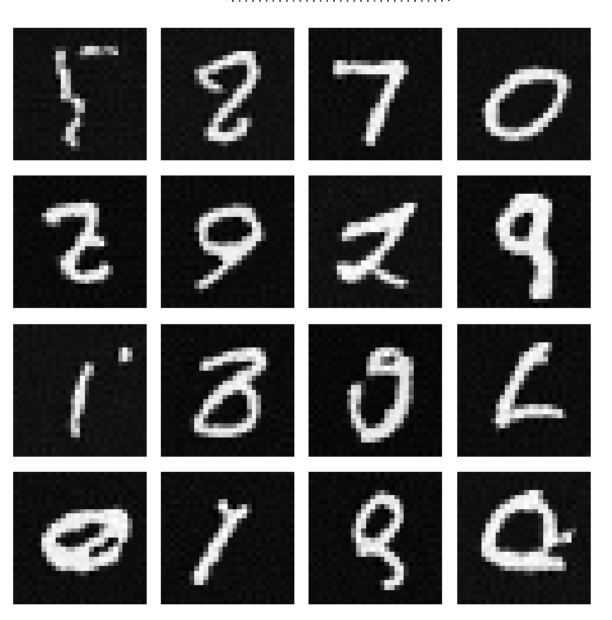
Ok, so: the numbers look even worse now. Take me back to the GAN 😿
- BUT: new shapes do pop up. As the literature says, diffusion models are more generalizable, while the GAN pretty much copies the dataset
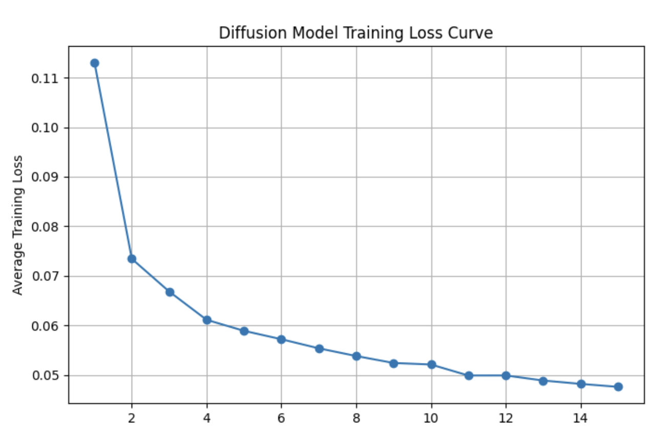
This is because I implemented a DDPM, where the P stands for probabilistic. More on that in the next section. Also the loss curve does not look like a Californian seismograph 🙏🙏🙏
future Adventures
Overall this experiment was a lot of fun. I learned a lot about the inner workings of image generation models and pros and cons of each. I especially learned more about how to put together a model when faced with just a description of the architecture.
DDIM Sampling?
What I implemented was a DDPM (Denoising Diffusion Probabilistic Model), as mentioned earlier. These model types sample random noise at every single step. They take way longer to generate images (usually thousands of denoising steps). DDIM (Denoising Diffusion Implicit Models) simplifies the reverse process specifically to make it much faster.
- Instead of sampling random noise every single time, you deterministically add noise. Thus, the same initial noise leads to the same generated image.
- This means more like 20-50 steps. A big improvement!
- But: this also means less variety. Predictable models are less fun 😼
Other ideas
- Trying to experiement with a different dataset other than MNIST. CIFAR 10 maybe?
- going to therapy